
정밀부품 공차 누적:
3D 조립 간극과 간섭 설계
정밀부품 공차 누적은 개별 부품의 치수 편차가 조립 기능에 어떤 영향을 주는지 평가하는 문제입니다. 플레이트와 스페이서가 각각 도면에 합격해도, 조합된 길이가 설치 공간보다 커지면 조립되지 않습니다. 반대로 간극이 너무 크면 위치결정과 지지 기능이 달라질 수 있습니다.
아래 3D 도해에서 부품 치수와 조립 상태를 바꾸면 이 차이를 직접 확인할 수 있습니다. 본문은 같은 예시를 최악조건, 통계적 분석, 기준면 설계와 검사까지 연결합니다. 예시 치수는 계산 관계를 설명하기 위한 가정값입니다.
부품은 합격인데, 왜 조립이 안 될까요?
치수 편차를 바꾸면 3D 조립 상태와 최종 간극이 함께 달라집니다.
3D 가속을 사용할 수 없어 정적 설계도를 표시합니다. 치수 계산은 계속 사용할 수 있습니다.
드래그로 회전 · 방향키로 회전 · Home 키로 시점 초기화
동작 줄이기 설정에 따라 애니메이션은 정지됩니다.
계산 간극 G
설계 범위
가정한 간극 요구 범위 안에 있습니다.
부품별 치수 편차
3D는 실제 치수 비율입니다. 미세 간극은 별도 확대 단면에서 확인하세요.
모든 개별 치수는 설정 공차 내
축방향 강체 간극을 설명하는 가정 모델입니다. 탄성변형·온도·형상오차는 포함하지 않습니다.
기능에서 시작하는 공차
간극·위치·접촉처럼 조립에서 필요한 기능을 먼저 정한 뒤 치수 사슬을 구성합니다.
최악조건과 확률의 구분
최악조건은 허용 범위의 끝값을, 통계적 분석은 명시한 분포와 공정 가정을 평가합니다.
도면·제조·검사의 연결
기준면, 가공 공정, 측정 조건과 조립 조정 방법을 하나의 검증 체계로 연결합니다.
01조립 기능과 치수 사슬
개별 치수와 조립 기능의 차이
정밀부품 공차 누적 문제는 개별 검사에서 모두 합격한 부품을 조립할 때 드러나기도 합니다. 각각의 길이가 도면 범위에 들어오더라도, 여러 길이의 합과 차이로 정해지는 최종 간극까지 자동으로 합격하는 것은 아닙니다. 조립 기능을 관리하려면 부품의 치수와 함께 완성 조립체가 확보해야 할 여유를 먼저 정의해야 합니다.
간극은 부품이 들어가기 위한 빈 공간에만 해당하지 않습니다. 축방향 유격, 커버와 내부 부품 사이의 여유, 센서와 타깃의 거리, 스프링의 설치 높이처럼 서로 다른 기능을 표현할 수 있습니다. 간극이 너무 작으면 간섭이나 예압 증가가 생기고, 너무 크면 흔들림과 위치 불안정이 생길 수 있으므로 양쪽 한계를 함께 살펴봅니다.
하우징과 세 부품의 축방향 모델
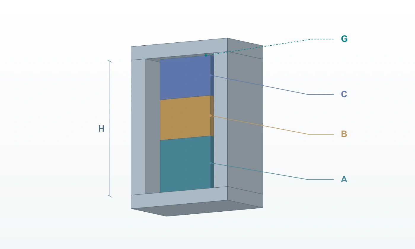
이 글은 하우징 내부 높이 H 안에 부품 A·B·C가 같은 축을 따라 놓이는 가상 조립체를 사용합니다. 바닥 기준면에서 차례로 맞닿은 세 부품의 합과 하우징 높이의 차이가 상단 간극 G입니다. 부품은 강체이고 접촉면은 평행하며, 이물·탄성 압축·코팅·온도 변화가 없는 상태를 기본 모델로 삼습니다.
| 항목 | 공칭값과 허용차 | 모델에서의 역할 |
|---|---|---|
| 하우징 H | 50.00 ± 0.05 mm | 사용할 수 있는 내부 높이 |
| 부품 A | 20.00 ± 0.03 mm | 적층 길이의 첫 번째 항 |
| 부품 B | 15.00 ± 0.02 mm | 적층 길이의 두 번째 항 |
| 부품 C | 14.90 ± 0.04 mm | 적층 길이의 세 번째 항 |
| 조립 간극 G | 요구 범위 0.05–0.15 mm | 부품 길이로부터 계산하는 기능 특성 |
공칭 간극은 50.00 − 20.00 − 15.00 − 14.90 = 0.10 mm입니다. 요구 범위의 중심에 있으므로 공칭 CAD 조립에서는 문제가 보이지 않습니다. 그러나 공칭값은 하나의 대표 상태일 뿐이며, 각 부품이 허용 범위 안에서 변할 때의 조립 결과를 검토해야 설계 여유를 판단할 수 있습니다.
모델 가정과 실제 조립 조건
위 수치는 원리를 설명하기 위한 가정값이며 특정 고객의 도면이나 납품품의 실측 사양이 아닙니다. 화면의 움직이는 3D 설계도는 선택한 치수에서 부품의 상대 위치와 간극을 계산해 보여 줍니다. 단면·분해·확대 표현은 이해를 돕는 시각화이며, 실제 탄성 접촉 해석이나 생산 합격률 시험을 대신하지 않습니다.
실제 적용에서는 무엇을 고정하고 무엇이 움직이는지, 어느 면이 먼저 닿는지부터 확인합니다. 하우징 바닥이 위치결정 기준인지, 상단 커버가 체결력으로 부품을 누르는지에 따라 기능이 달라집니다. 같은 음의 간극이라도 의도된 압입·예압 설계와 우발적 조립 간섭은 다르며, 필요한 하중과 변형 검증도 구분해야 합니다.
따라서 출발점은 모든 치수에 작은 공차를 붙이는 작업이 아닙니다. 사용 상태에서 필요한 기능 범위를 정하고, 그 기능을 지배하는 접촉면과 치수 경로를 연결하는 작업입니다. 이후 최악조건, 통계 분석, 도면 기준계와 검사 방법을 같은 기능 모델에 맞추면 부품 합격과 조립 합격 사이의 빈틈을 줄일 수 있습니다.
부호가 있는 치수 사슬
축방향 공차 누적은 먼저 닫힌 치수 경로를 한 바퀴 따라가며 정리할 수 있습니다. 기준면에서 하우징 상단으로 가는 높이는 간극을 늘리고, 그 안을 채우는 부품 높이는 간극을 줄입니다. 이 모델의 기능식은 G = H − A − B − C이며, 모든 항은 같은 단위와 같은 방향 기준으로 작성합니다.
부호는 도면의 화살표가 향하는 방향을 기계적으로 복사해서 결정하지 않습니다. 해당 치수를 조금 키웠을 때 기능 간극이 늘어나는지 줄어드는지 확인하면 이해하기 쉽습니다. H를 키우면 G가 커지고, A·B·C를 키우면 G가 작아지므로 감도는 각각 +1, −1, −1, −1입니다.
기준면에서 접촉면까지의 경로
치수 경로에는 실제 접촉 상태를 결정하는 면만 포함합니다. 예를 들어 부품의 외형 전체 길이가 길어져도 조립 위치를 정하는 어깨면 사이 거리가 변하지 않으면 해당 외형 치수는 이 간극의 직접 항이 아닙니다. 반대로 도면에서 작게 표시된 와셔 두께라도 축방향 접촉 경로 안에 있으면 반드시 반영해야 합니다.
공칭 치수와 실제 편차를 분리하면 계산을 검토하기 쉽습니다. H = H₀ + δH와 같은 표현을 사용하면 간극 편차는 δG = δH − δA − δB − δC가 됩니다. 공칭값을 바꾸는 설계 수정과 공정 변동을 줄이는 개선은 이 식에서 서로 다른 역할을 하므로 따로 기록하는 것이 좋습니다.
치수 사슬의 항이 많다고 해서 도면의 모든 치수를 더하면 안 됩니다. 같은 물리적 거리를 전체 길이와 부분 길이로 중복 포함하면 실제보다 큰 누적량을 계산할 수 있습니다. 반대로 측정 기준이 다른 두 거리를 같은 출발점으로 취급하면 누락된 위치 편차가 생깁니다. 경로를 그림으로 그린 뒤 식과 일대일로 대응시키는 절차가 유용합니다.
선형 모델과 계산 검증
기울기, 회전, 유격 이동과 접촉점 전환이 작으면 감도를 이용한 선형 근사가 유용합니다. 그러나 부품이 기울어 한쪽 모서리부터 닿거나 체결하면서 휘는 경우에는 하나의 길이 합으로 접촉 상태를 설명하기 어렵습니다. 먼저 축방향 기본 모델을 검증하고, 기능에 영향을 주는 자유도만 단계적으로 확장해야 해석과 검사 결과를 연결할 수 있습니다.
단위 관리도 치수 사슬의 일부입니다. 길이는 mm, 각도는 rad 또는 명시된 각도 단위로 통일하고, 각도 편차를 길이로 환산할 때는 실제 레버 암을 사용합니다. 가공 공차를 µm로 받고 조립 요구를 mm로 입력하는 경우에는 변환 단계를 분리해 기록하면 천 배의 입력 오류를 예방하기 쉽습니다.
계산식의 검증에는 단순한 극단값 시험이 효과적입니다. H만 늘렸을 때 간극이 늘어나는지, A만 늘렸을 때 간극이 줄어드는지, 모든 편차를 영으로 돌리면 0.10 mm가 되는지 확인합니다. 3D 설계도와 표의 숫자가 같은 식을 사용하도록 연결하면 시각적으로 그럴듯하지만 계산 방향은 잘못된 모델을 걸러낼 수 있습니다.
02최악조건과 통계적 분석
상한·하한과 최악조건
최악조건 분석은 허용 범위 안의 치수 조합이 만들 수 있는 기능값의 경계를 구합니다. 독립적인 직사각형 허용영역과 현재의 선형식을 전제로 하면, 간극을 가장 작게 만드는 조합은 하우징이 최소이고 세 부품이 모두 최대인 상태입니다. 간극을 가장 크게 만드는 조합은 그 반대이며, 발생 빈도를 가정할 필요가 없습니다.
최소 간극은 49.95 − 20.03 − 15.02 − 14.94 = −0.04 mm입니다. 각 치수는 자신의 도면 범위 안에 있지만, 쌓인 부품은 하우징 내부 높이보다 0.04 mm 큽니다. 강체 모델에서는 이 상태를 조립 가능한 틈으로 해석할 수 없으며, 간섭 또는 추가 변형을 요구하는 상태로 구분합니다.
공칭 합격과 전 조합 합격의 차이
| 상태 | 치수 조합 | 간극 G | 요구 범위 판정 |
|---|---|---|---|
| 공칭 | 모든 항이 공칭값 | 0.10 mm | 범위 안 |
| 최소 간극 | H 최소, A·B·C 최대 | −0.04 mm | 간섭 |
| 최대 간극 | H 최대, A·B·C 최소 | 0.24 mm | 상한 초과 |
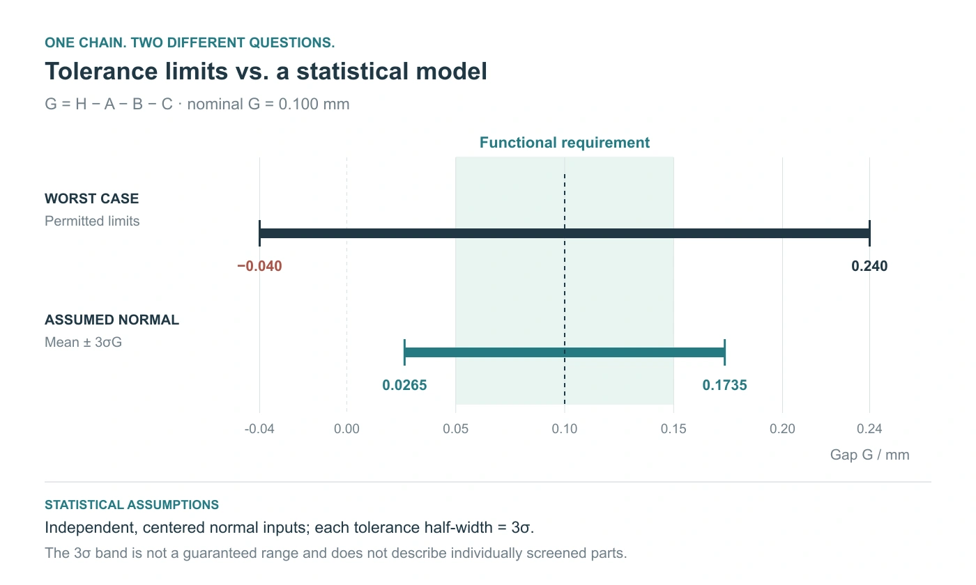
| 최악조건 전체 범위 | 허용 편차를 경계까지 반영 | −0.04–0.24 mm | 요구 0.05–0.15 mm를 벗어남 |
대칭 양측 공차에서는 이 예시의 최악조건 반폭이 0.05 + 0.03 + 0.02 + 0.04 = 0.14 mm입니다. 따라서 공칭값 0.10 mm를 중심으로 ±0.14 mm가 됩니다. 여기서 더하는 값은 공차 구간 전체 폭이 아니라 각 항의 편측 허용차이며, 폭과 반폭을 혼용하면 누적량이 두 배로 달라집니다.
최악조건 범위를 요구 안에 넣으려면 공칭 위치와 변동 폭을 모두 살펴야 합니다. 이 예시에서 공칭 간극만 늘리면 최소값은 개선되지만 최대값도 같은 만큼 커집니다. 폭이 0.28 mm인 결과 범위를 폭이 0.10 mm인 요구 안으로 이동만 시켜 넣을 수 없으므로, 공차 축소나 구조 변경·조정 수단이 필요합니다.
비대칭 공차와 교환성
편측 공차나 비대칭 공차가 있을 때는 각 항의 실제 상한과 하한을 사용합니다. 예를 들어 하한은 고정하고 상한만 허용하는 두께를 ±공차처럼 취급하면 공칭 중심부터 잘못 해석할 수 있습니다. 선형식에서는 항의 부호에 따라 해당 상한과 하한을 선택하고, 비선형 접촉 조건에서는 경계 조합과 내부 극값을 별도로 확인합니다.
최악조건 불합격은 모든 조립품이 불합격이라는 뜻은 아닙니다. 현재 도면만으로 허용되는 모든 조합의 기능 합격을 보장할 수 없다는 뜻입니다. 반대로 최악조건 계산이 요구 안에 들어와도 모델에서 누락한 기울기·버·온도·측정 오류가 사라지는 것은 아니므로, 계산의 적용 범위와 실제 검증 조건을 함께 관리해야 합니다.
안전 여유가 작거나 임의 교환성이 필요한 조립에서는 최악조건 검토의 가치가 큽니다. 수리 현장에서 다른 로트의 부품을 섞거나 교체 부품을 장기간 공급하면 처음의 생산 분포가 그대로 유지되지 않을 수 있습니다. 통계적으로 양호한 초기 생산 결과와 도면이 허용하는 교환성을 서로 다른 승인 항목으로 다루는 것이 합리적입니다.
RSS 계산과 통계 가정
RSS는 여러 변동의 제곱합에 제곱근을 취하는 방식입니다. 선형식 G = H − A − B − C에서 각 치수의 변동이 서로 독립이면 분산은 σG² = σH² + σA² + σB² + σC²가 됩니다. 표준편차의 결합식 자체는 정규분포를 요구하지 않지만, 그 결과를 특정 합격률로 바꾸려면 출력 분포에 대한 추가 가정이 필요합니다.
도면 공차는 허용 범위이고 표준편차는 공정 데이터의 산포입니다. 따라서 ±0.05 mm라는 도면만 보고 σ가 0.05 mm이거나 0.05/3 mm라고 확정할 수 없습니다. 본 예시의 통계 계산은 설명을 위해 각 편측 허용차를 3σ로 놓고, 평균이 공칭에 있으며 치수가 서로 독립적인 정규분포라고 명시적으로 가정합니다.
분산 결합과 기능 합격률의 구분
| 계산 항목 | 가정에 따른 값 | 해석 |
|---|---|---|
| 입력 σ | 각 편측 허용차 ÷ 3 | 도면만으로 확인되는 실측값이 아님 |
| 결합 σG | 약 0.02449 mm | 독립 변동의 결합 표준편차 |
| 출력 3σ 반폭 | 약 0.07348 mm | 공칭 중심의 통계적 폭 |
| 출력 중심 ±3σ | 약 0.02652–0.17348 mm | 요구 범위와 별개의 구간 |
| 요구 범위 예측 합격률 | 약 95.88% | 무선별 정규 모집단 가정에 따른 계산 |
계산하면 σG = √[(0.05/3)² + (0.03/3)² + (0.02/3)² + (0.04/3)²] ≈ 0.02449 mm입니다. 같은 가정에서 3σG는 약 0.07348 mm입니다. 이 값이 최악조건 반폭 0.14 mm보다 작다는 사실은 산포 모델의 차이를 보여 줄 뿐, 도면에서 가능한 극단 조합이 없어졌다는 뜻은 아닙니다.
요구 간극은 0.05–0.15 mm이므로 평균 0.10 mm에서 허용되는 거리는 양쪽 0.05 mm입니다. 정규 누적분포로 이 구간의 확률을 계산하면 약 95.88%가 됩니다. 출력의 ±3σ 구간과 실제 요구 구간이 같지 않으므로, 입력에서 3σ를 사용했다는 이유만으로 조립 합격률을 약 99.73%라고 말할 수 없습니다.
선별 조건과 생산 데이터
이 확률은 공차 밖 꼬리도 포함하는 무선별 정규 모집단을 대상으로 한 가정 계산입니다. 단품을 전수 검사해 공차 합격품만 조립한다면 입력은 선별 조건을 받은 분포가 됩니다. 그때의 조립 합격률은 조건부 분포로 다시 계산해야 하며, 앞의 95.88%를 그대로 현장 수율이나 합격 부품끼리의 조립률로 옮기면 안 됩니다.
통계 분석의 입력에는 공정별 실제 평균과 표준편차, 로트 구분, 표본 크기와 측정 조건이 필요합니다. 한 번의 양호한 샘플에서 얻은 작은 산포를 장기간 공정의 대표값으로 쓰면 평균 이동과 로트 간 차이가 가려질 수 있습니다. 설계 가정과 생산 데이터가 얼마나 다른지 확인하고 모델을 갱신해야 RSS가 원가와 품질 판단에 도움이 됩니다.
3D 슬라이더는 허용 범위 안에서 선택한 조합의 간극을 직접 계산하는 도구입니다. 슬라이더를 여러 번 움직이거나 자동 애니메이션을 반복한 횟수는 무작위 표본 수가 아니며, 색상 변화 비율도 생산 합격률이 아닙니다. 결정론적 조립 검토와 통계적 모집단 예측을 분리하면 시각화의 장점을 유지하면서 해석을 과장하지 않을 수 있습니다.
03분포·상관과 시뮬레이션
평균 이동·상관·분포 형태
같은 산포를 가진 공정이라도 평균이 요구 구간의 중심에서 벗어나면 합격률이 달라집니다. 예시 모델의 평균 간극은 μG = μH − μA − μB − μC입니다. A의 공정 평균만 커지면 간극 평균은 그만큼 작아지므로, 표준편차가 일정하더라도 하한 쪽 위험은 증가합니다. 공차 누적에서는 중심과 산포를 함께 추적해야 합니다.
공구 마모, 보정값 변경, 소재 로트와 작업 온도는 시간에 따라 평균을 움직일 수 있습니다. 이런 데이터를 모두 섞어 히스토그램 하나로 만들면 서로 다른 상태가 하나의 넓은 분포처럼 보일 수 있습니다. 반대로 매우 짧은 구간만 분석하면 로트 간 이동이 누락되므로, 분석하려는 공급 기간과 교체 부품 범위에 맞게 데이터를 나눕니다.
상관과 치수 감도의 부호
서로 다른 치수가 같은 소재·설비·온도 영향을 받으면 독립성을 가정하기 어려울 수 있습니다. 일반적인 선형 분산식은 σG² = Σ(si²σi²) + 2Σ(i<j)si·sj·Cov(Xi,Xj)입니다. 여기서 si는 치수 감도이며, 공분산 항에는 그 부호가 함께 들어갑니다. 상관계수만 보고 최종 산포의 증감을 판단해서는 안 됩니다.
이 예시에서 A와 B가 함께 커지는 양의 상관은 두 항이 모두 간극을 줄이므로 간극 산포를 키우는 방향입니다. 반면 H와 A가 같은 양만큼 함께 커진다면 두 변화가 기능식에서 상쇄될 수 있습니다. 따라서 양의 상관이 항상 불리하다고 단정하지 말고, 원인과 감도 부호, 실제 상관의 크기를 함께 검토해야 합니다.
공통 오차가 상쇄되는 구조라도 생산과 조립 경로가 달라지면 그 관계가 유지되지 않을 수 있습니다. 같은 장비에서 함께 가공한 짝 부품은 상관이 있어도, 창고에서 무작위로 섞거나 다른 공급처 부품으로 교체하면 짝 관계가 사라집니다. 상관을 설계 여유로 사용할 때는 로트·짝 관리와 서비스 교환 방식까지 조건으로 남겨야 합니다.
생산 분포와 데이터 해석
공정 데이터는 정규분포 외에도 비대칭·다봉·절단 분포를 보일 수 있습니다. 공구 보정 주기, 기계 여러 대의 혼합, 선별 검사와 재작업은 분포 모양을 바꾸는 대표적인 조건입니다. 표본 평균과 표준편차가 같아도 요구 한계 근처의 꼬리 확률은 다를 수 있으므로, 히스토그램과 시간 순서 자료를 함께 검토합니다.
Cp와 Cpk는 안정된 공정과 적절한 분포 해석을 전제로 치수 요구에 대한 공정 위치와 산포를 요약합니다. 높은 지수가 치수 사슬에 빠진 항을 찾아 주거나 조립 모델의 정확성을 보증하지는 않습니다. 지수의 계산 기간과 표준편차 추정 방식도 남겨야 서로 다른 로트·공정의 숫자를 같은 의미로 비교할 수 있습니다.
실무에서는 먼저 공정별 데이터가 같은 조건을 대표하는지 확인하고, 평균 이동·상관·비정규성을 차례로 검토합니다. 불확실한 항목은 유리한 쪽으로 가정하기보다 민감도 시나리오로 남겨 결과가 얼마나 달라지는지 확인합니다. 데이터가 부족한 단계에서는 최악조건 경계와 통계 가정의 결과를 나란히 제시하는 편이 의사결정에 도움이 됩니다.
몬테카를로와 비선형 조립
몬테카를로 분석은 정의한 입력 분포에서 치수 조합을 반복 추출하고 기능식을 계산하는 방법입니다. 입력이 복잡하거나 출력이 비선형일 때 간극의 분포와 한계 초과 패턴을 살펴보는 데 유용합니다. 그러나 반복 횟수를 늘려도 잘못된 분포·누락된 상관·틀린 접촉 모델이 자동으로 수정되지는 않으며, 결과의 타당성은 입력과 모델에 달려 있습니다.
현재의 G = H − A − B − C는 선형식이므로 독립 정규분포 가정에서는 평균과 분산을 직접 계산할 수 있습니다. 이때 시뮬레이션은 해석식을 대체할 필요가 없으며, 구현이 같은 결과로 수렴하는지 확인하는 검증 수단이 됩니다. 입력 평균·표준편차와 단위를 의도적으로 바꾸는 시험을 함께 수행하면 모델 연결 오류를 발견하기 쉽습니다.
표본 수와 드문 불합격
표본 수는 표시되는 소수점 자릿수와 별개입니다. 아주 드문 불합격을 평가하려면 그 사건이 나타날 만큼 충분한 표본과 적절한 불확도 평가가 필요합니다. 제한된 시행에서 불합격이 한 번도 없었다고 실제 위험이 영이라고 결론내릴 수 없으며, 필요한 신뢰 수준과 허용 위험에 맞춰 결과를 해석해야 합니다.
재현 가능한 분석에는 입력 분포와 근거 데이터, 난수 시드, 시행 수, 소프트웨어 버전과 판정식을 기록합니다. 같은 모델을 다시 실행했을 때 결과 차이가 예상되는 표본 변동 안에 있는지도 확인합니다. 중요한 설계 변경은 평균이나 합격률 하나만 비교하지 않고, 상·하한 초과의 원인과 해당 치수 조합을 함께 추적합니다.
단품 전수 선별을 모델링할 때는 불합격 입력을 제외하거나 조건부 분포를 사용해야 합니다. 다만 단순 제외가 현장의 선택 조립을 모두 표현하지는 않습니다. 크기별 구간을 나눠 짝을 맞추거나 특정 로트끼리 조립하면 입력 간 의존성이 새로 생기므로, 실제 재고 배정과 짝 선정 규칙을 모델 안에 반영해야 합니다.
접촉 상태와 3D 해석
두 개 이상의 가이드, 위치결정 핀, 기울어진 면과 유연한 부품이 있으면 조립 접촉점이 치수에 따라 바뀔 수 있습니다. 이때 최소 간극은 단순 평균 위치가 아니라 특정 모서리나 국부 영역에서 발생합니다. 선형화 기준점 주변만 살피는 모델과 실제 3D 접촉 모델의 차이를 이해하고, 필요한 경우 제한된 구간에서 별도 검증을 수행합니다.
체결력에 따른 변형이 기능을 지배하면 재료 강성, 접촉 조건과 하중 경로도 필요합니다. 공차 모델이 계산한 음의 간극에 임의의 힘을 대응시키거나, 화면에서 부품이 겹치는 양을 실제 압축량이라고 단정해서는 안 됩니다. 형상 편차 해석과 구조 해석을 연결하되, 마찰·접촉·경계조건의 가정을 분리해 관리합니다.
움직이는 설계도는 공칭 조립, 최소 간극과 최대 간극을 같은 시점과 기준면에서 비교할 때 특히 유용합니다. 치수 슬라이더 하나가 어느 면을 이동시키는지 확인하고, 단면에서 간섭 위치를 살펴보면 수식의 부호를 직관적으로 이해할 수 있습니다. 이후 실제 도면 검토와 계측 데이터로 모델을 보완하는 순서가 효과적입니다.
04기준면과 기하공차
기준면과 치수 기입 방식
같은 형상을 표현하더라도 치수를 연결하는 방식에 따라 허용되는 위치 관계가 달라질 수 있습니다. 연속 치수는 앞선 형상에서 다음 형상까지의 거리를 이어 가고, 기준 치수는 여러 형상을 공통 기준에서 정의합니다. 설계 의도가 특정 두 면 사이의 기능 간극에 있다면, 그 관계가 어떤 치수와 공차로 실제 제한되는지 확인해야 합니다.
연속 치수에서 끝 위치는 중간 구간들의 합으로 정해지므로 각 구간의 허용 편차가 반영됩니다. 공통 기준 방식은 개별 위치를 기준에서 직접 제한할 수 있지만, 임의의 두 위치 사이 거리에는 두 위치 편차의 차이가 남습니다. 기준 치수로 바꾸기만 하면 모든 공차 누적이 사라진다는 설명은 실제 기능 관계를 단순화한 것입니다.
설계·가공·검사의 기준 정합성
| 방식 또는 조건 | 설계상 장점 | 추가 확인 항목 |
|---|---|---|
| 연속 치수 | 인접 기능 구간을 직접 표현 | 끝 위치까지의 누적과 중복 치수 |
| 공통 기준 치수 | 여러 위치를 한 기준에 연결 | 두 위치 사이 상대 거리의 허용 범위 |
| 기능 기준면 | 실제 조립 접촉과 도면을 연결 | 기준면의 형상·접촉·구속 상태 |
| 가공 기준 전환 | 공정별 접근과 고정에 대응 | 재세팅으로 생기는 위치 관계의 변화 |
| 검사 기준계 | 판정 결과를 일관되게 비교 | 도면 기준의 구현과 정렬 방법 |
좋은 기능 기준은 조립체가 실제로 위치를 정하는 면·축·형상과 연결됩니다. 평평해 보이는 큰 면이 반드시 최선의 기준은 아니며, 사용 상태에서 닿지 않는 외관면을 기준으로 삼으면 기능 면까지 불필요한 경로가 생길 수 있습니다. 또한 기준면 자체의 평면도와 접촉 안정성이 나쁘면 기준을 지정해도 반복 위치가 흔들릴 수 있습니다.
가공에서는 접근성 때문에 설계 기준과 다른 면을 잡는 경우가 있습니다. 그 자체가 잘못은 아니지만, 첫 세팅에서 만든 형상을 두 번째 세팅에서 다시 위치시키는 과정의 관계를 관리해야 합니다. 완성 치수만 개별 측정하고 세팅 간 기준 전환을 놓치면, 각각 맞는 구멍과 면이 서로 잘못된 위치 관계를 가질 수 있습니다.
검사 기준과 도면 개정
검사 정렬도 기능을 반영해야 합니다. 모든 면에 가장 잘 맞도록 자유롭게 최적 맞춤을 수행하면 실제 조립 기준에서 보이는 오차 일부가 줄어 보일 수 있습니다. 도면이 요구하는 기준 순서와 구속 조건을 구현한 정렬인지, 탐색 목적의 최적 맞춤인지 구분하고 결과 보고서에 사용한 기준계를 남깁니다.
한 기능 치수를 여러 중복 치수로 동시에 엄격하게 제한하면 가공과 검사에서 상충하는 요구가 생길 수 있습니다. 전체 길이와 각 구간 길이의 허용 범위를 모두 독립 요구로 둘 경우, 단순히 구간 상한을 더한 조합이 전체 길이 조건 때문에 허용되지 않을 수도 있습니다. 도면의 독립 요구와 참고 치수를 명확히 나누고 모델도 그 제약을 반영해야 합니다.
도면 수정은 치수 화살표의 배치 변경에 그치지 않습니다. 기능 기준을 바꾸면 가공 고정, 검사 정렬, 성적서 항목과 협력사 해석도 함께 달라질 수 있습니다. 개정 전후의 기능식과 허용영역을 비교하고, 바뀐 기준에서 기존 측정값을 그대로 사용할 수 있는지 확인해야 설계 개선이 생산 단계까지 이어집니다.

형상·위치·기울기와 국부 간섭
길이 공차만으로 모든 조립 불량을 설명할 수는 없습니다. 평균 두께가 맞아도 면이 휘거나 두 면이 평행하지 않으면 실제 접촉점의 높이가 달라집니다. 구멍 지름이 맞아도 위치와 축 방향이 틀리면 핀이 들어가지 않을 수 있습니다. 크기, 형상, 방향과 위치를 기능에 맞게 구분해서 도면과 검사 항목에 연결해야 합니다.
적층 부품에서는 상단 간극이 한 값이 아니라 위치에 따른 함수가 될 수 있습니다. 두 면 사이에 작은 기울기 θ가 있으면 거리 L만큼 떨어진 위치의 높이 차이는 작은 각도에서 대략 Lθ로 표현됩니다. 각도는 라디안으로 사용하며, 실제 최소 간극은 기준점의 간극에서 가장 불리한 국부 높이 변화를 반영해 검토합니다.
치수 합격과 형상 합격의 결합
평면도는 한 면의 형상, 평행도는 기준에 대한 방향 관계, 위치도는 형상 위치의 허용영역을 다루는 등 역할이 다릅니다. 어떤 공차를 적용할지는 기능과 채택한 도면 규격에 따라 결정합니다. 서로 다른 규격 체계의 기호나 기본 해석을 섞어 쓰거나, 형상 공차 하나가 모든 조립 조건을 대신한다고 가정하지 않습니다.
재료 조건 수정자와 데이텀 이동을 사용하는 도면은 단순 ±길이 표보다 복잡한 허용영역을 가질 수 있습니다. 추가 허용량은 기호와 적용 조건이 허용하는 경우에만 생기며, 모든 구멍과 핀에 임의로 더하는 여유가 아닙니다. 조립 여유를 계산할 때는 크기와 위치의 결합 조건, 실제 위치결정 방식과 경계 조건을 함께 해석해야 합니다.
사각 구멍과 상대 부품에서는 직선 벽 사이 폭이 충분해도 코너에서 먼저 간섭할 수 있습니다. 이는 전체 폭의 공차 누적과 별개로 내부 R과 외부 모서리의 형상 관계가 작용하기 때문입니다. 이런 경우는 와이어 방전가공 내부 코너와 조립 간섭처럼 국부 형상을 따로 검토해야 해결 방향이 명확해집니다.
구속 상태와 검사 위치
얇은 플레이트나 긴 부품은 고정 방법에 따라 모양이 달라집니다. 강하게 눌러 측정하면 자유 상태의 휨이 작아 보일 수 있고, 조립 체결 후에는 접촉면을 따라 다른 형상이 될 수 있습니다. 기능이 어느 상태에서 필요한지 정한 뒤 자유 상태, 지지 상태와 체결 상태의 판정 조건을 구분해야 합니다.
가공면의 거칠기, 국부 돌기와 버는 도면상의 이상적인 면과 실제 접촉 위치를 다르게 만듭니다. 첫 체결에서 돌기가 눌리거나 자리를 잡으면 이후의 조립 높이도 달라질 수 있습니다. 치수 사슬에 무조건 일정 보정값을 더하기보다 접촉면 상태를 관리하고, 반복 체결과 사용 하중에서 기능 치수가 유지되는지 확인합니다.
형상과 위치를 포함한 검사는 기능 면의 여러 지점과 실제 조립 경로를 확인해야 합니다. 한 점의 두께 측정이나 단일 단면의 간극으로 전체 면을 대표하면 국부 최소값을 놓칠 수 있습니다. 측정할 위치와 정렬, 공간 분해능을 필요한 결함 크기에 맞추고, 시각화에서 찾은 위험 구역을 실제 검사 계획에 반영합니다.
05제조·검사와 공차 배분
제조 상태·온도·표면과 측정
공차 누적 계산에 사용하는 치수는 어느 공정 단계의 값인지 분명해야 합니다. 열처리 전 길이, 코팅 전 두께와 최종 세정 후 조립 치수를 섞으면 같은 식에서도 다른 상태를 계산하게 됩니다. 기능을 승인하는 기준은 원칙적으로 지정된 최종 상태이며, 공정 중 치수는 그 상태에 도달하기 위한 관리값으로 구분합니다.
절삭과 열처리는 잔류응력과 형상에 영향을 줄 수 있으며, 고정 중에는 보이지 않던 변형이 클램프를 풀거나 재료를 제거한 뒤 나타날 수 있습니다. 이때 한 점의 길이만 보정하면 전체 면 관계가 해결되지 않을 수 있습니다. 가공 순서와 충분한 안정화, 측정 시점과 지지 방법을 최종 기능 조건에 맞춰 검토합니다.
온도와 표면층의 치수 경로
| 변화 요인 | 간극에 미치는 경로 | 관리 기준 |
|---|---|---|
| 온도 변화 | 재질·길이·온도에 따른 항별 팽창 | 기준 온도, 사용 온도와 온도 구배 |
| 코팅·도금 | 기능 면의 최종 위치 변화 | 어느 면에 얼마나 형성되는지와 최종 치수 |
| 버·입자·잔류물 | 국부 들뜸과 접촉점 변화 | 청정도와 디버링, 조립 전 확인 |
| 가공·체결 변형 | 자유 상태와 구속 상태의 형상 차이 | 측정 지지와 사용 하중 조건 |
| 측정 불확도 | 판정값의 신뢰 범위 | 측정 모델과 합의된 판정 규칙 |
일차 열팽창 모델에서는 간극 변화가 ΔG ≈ αH·H·ΔTH − αA·A·ΔTA − αB·B·ΔTB − αC·C·ΔTC로 표현됩니다. α는 해당 재질과 온도 범위의 선팽창계수입니다. 모든 부품이 같은 재질이고 같은 온도 변화를 받으면 공통 팽창이 상당 부분 상쇄되지만, 재질 차이와 온도 구배가 있으면 그 단순화가 성립하지 않습니다.
표면처리는 명목 도금 두께를 모든 치수에 한 번 더하는 방식으로 처리하지 않습니다. 적층 부품의 두 기능 면에 층이 생기면 그 두께 합이 적층 높이를 바꿀 수 있고, 하우징 내부 면의 층은 사용 가능한 공간을 줄일 수 있습니다. 도면이 이미 최종 치수를 지정했다면 같은 코팅 영향을 다시 더하지 않도록 치수 정의를 확인합니다.
접촉 재현성과 검사 판정
버와 이물은 균일한 표면층처럼 거동하지 않습니다. 한쪽에 남은 작은 돌기가 부품을 기울게 하면 입자 높이보다 먼 위치에서 큰 간극 차이가 나타날 수 있습니다. 조립 전 청정도는 외관 관리만의 문제가 아니며, 정밀부품 세정과 청정도 관리에서 다루는 잔류물과 재오염 조건도 실제 접촉의 재현성에 연결됩니다.
측정 불확도는 부품이 실제로 변하는 생산 산포와 다른 개념입니다. 온도 보정, 측정력, 정렬, 장비 교정과 반복성은 보고한 치수에 대한 신뢰 범위에 영향을 줍니다. 측정 데이터로 공정 산포를 추정할 때는 측정계의 기여를 검토하고, 같은 오차를 공정 변동과 검사 여유에 중복 반영하지 않도록 모델을 구분합니다.
한계에 가까운 값의 합격 여부는 측정값만으로 자명하지 않을 수 있습니다. 발주 전에 측정 방법과 불확도, 경계값의 판정 규칙을 합의하면 공급자와 사용자의 판단 차이를 줄일 수 있습니다. 최종 조립 간극을 직접 측정하는 검사는 개별 치수의 합성 계산을 보완하지만, 접근성·측정력과 실제 사용 상태의 재현성도 검토해야 합니다.
공차 배분과 공정 원가
공차 배분은 조립 기능이 허용하는 변동을 각 부품에 나누는 설계 작업입니다. 모든 공차를 같은 비율로 줄이면 계산은 단순하지만, 공정 난이도와 검사 비용을 반영하지 못할 수 있습니다. 길이 감도, 현재 공정 산포, 가공 접근성과 형상 안정성, 필요한 수량을 함께 고려해야 현실적인 배분안을 만들 수 있습니다.
최악조건으로 요구 전 범위를 만족시키려면 공칭 위치가 적절할 뿐 아니라 감도 절댓값을 곱한 편측 허용차의 합이 기능 예산 안에 있어야 합니다. 본 예시의 공칭 0.10 mm와 요구 0.05–0.15 mm에서는 그 합이 0.05 mm 이하여야 합니다. 다만 이 허용 여유를 길이 공차에 모두 사용하면 다른 모델 오차에 남는 여유는 없습니다.
감도와 산포 기여도의 활용
| 항목 | 간극 감도 | 예시 분산 기여도 | 해석 |
|---|---|---|---|
| 하우징 H | +1 | 약 46.3% | 독립·각 편측 허용차 = 3σ 가정에서 가장 큰 항 |
| 부품 A | −1 | 약 16.7% | 부호는 방향, 제곱은 분산 기여를 결정 |
| 부품 B | −1 | 약 7.4% | 이미 작은 항을 더 줄일 때의 효과 검토 |
| 부품 C | −1 | 약 29.6% | H와 함께 산포 개선 후보로 검토 |
표의 비율은 실제 공정 능력 순위가 아니라 앞에서 정한 가정 모델의 결과입니다. H의 분산 기여가 크므로 H를 먼저 살펴볼 근거는 있지만, 그 가공이 매우 어렵다면 다른 항 개선이나 구조 변경이 더 경제적일 수 있습니다. 상관이 있으면 교차항도 생기므로 독립 모델의 기여도 표를 그대로 비용 우선순위로 사용하지 않습니다.
공차를 줄이는 방법에는 공구나 장비를 바꾸는 것 외에도 재세팅 횟수 축소, 공통 기준 유지, 안정된 접촉면 확보와 공정 순서 조정이 있습니다. 부품 수를 줄이거나 기능 높이를 한 번에 형성하도록 구조를 바꾸면 치수 경로 자체가 짧아질 수 있습니다. 다만 일체화는 접근성·열변형·수리성과 같은 새로운 제약도 만들 수 있으므로 함께 비교합니다.
전체 원가와 배분안 비교
공정 원가는 가공 시간만으로 결정되지 않습니다. 더 작은 공차가 온도 안정화, 추가 마감, 전수 측정, 재작업과 낮은 수율을 요구하면 전체 비용이 커집니다. 반대로 적절한 조정 구조는 부품 가공 부담을 낮출 수 있지만 조립 시간과 부품 관리 비용을 늘립니다. 동일한 기능 합격 기준에서 제조부터 서비스까지 비교해야 배분의 의미가 생깁니다.
통계적 배분을 선택할 때는 목표 합격률만 정하고 끝내지 않습니다. 필요한 공정 안정성, 평균 관리, 로트별 측정과 공급 변경 시 재검증 조건을 함께 정합니다. 생산량이 적어 산포 추정이 어려운 맞춤 부품은 충분한 데이터가 있는 양산품과 같은 가정을 적용하기 어려우므로, 기능 검사와 조정 전략의 비중을 다르게 가져갈 수 있습니다.
배분안을 비교할 때는 원래 모델, 수정 모델과 변경 이유를 나란히 남깁니다. 공칭값 변경으로 중심을 맞춘 것인지, 실제 산포를 줄인 것인지, 선별로 조합을 제한한 것인지 구분해야 합니다. 각각은 수율·교환성·검사 부담에 다른 영향을 주며, 같은 최종 간극을 만들더라도 장기 공급 조건은 달라질 수 있습니다.
06조립 조정과 도면 관리
심 조정·선택 조립·기능 검사
조정 구조는 남은 간극을 측정한 뒤 기능값을 목표 범위로 맞추는 방법입니다. 심, 조정 나사와 가변 스톱 등은 서로 다른 방향으로 기능 치수를 바꾸므로 위치와 작동 원리를 먼저 정의합니다. 조정 가능 범위가 충분한지뿐 아니라 체결 후 고정, 반복 사용 중 이동과 유지보수 절차까지 검토해야 합니다.
본 모델에서 부품 A·B·C와 같은 적층 경로에 두께 S의 심을 추가하면 간극은 G′ = G − S입니다. 양의 두께를 추가하면 간극이 줄어드므로 큰 간극을 줄이는 데 사용할 수 있습니다. 이미 음의 간극인 상태에 같은 위치의 심을 더하면 간섭이 커지며, 심은 위치와 방향을 무시한 만능 보정 수단이 아닙니다.
조정 방향과 잔여 오차
예를 들어 실측 간극이 0.14 mm인 가정 상태에서 0.04 mm 심을 적층 안에 넣으면 기하학적 목표는 0.10 mm가 됩니다. 그러나 실제 결과에는 심 두께 공차, 접촉면의 평행도와 측정 불확도가 남습니다. 심 선정 후 다시 조립하고 기능 간극을 확인하는 절차까지 포함해야 계산값과 완성 상태를 연결할 수 있습니다.
커버를 들어 올리는 스페이서는 하우징의 유효 높이를 늘릴 수 있으므로 적층 내부 심과 반대 방향으로 작용할 수 있습니다. 다만 그 변경은 볼트 물림, 씰 압축, 위치결정과 강성까지 바꿀 수 있습니다. 간극 하나가 좋아졌다는 이유로 승인 없이 다른 접촉 경로에 보정 부품을 추가하지 말고 전체 조립 요구를 다시 확인합니다.
선택 조립은 측정한 부품을 크기 구간별로 나누고 조합 규칙을 정해 기능 범위를 맞추는 방식입니다. 부품의 제조 공차를 유지하면서 조립 결과를 개선할 수 있지만, 어떤 부품이든 자유롭게 바꿔도 된다는 교환성을 제공하지는 않습니다. 분류 구간의 폭, 경계 판정과 짝 추적을 도면·공정 계획에 맞춰 관리해야 합니다.
재고 관리와 기능 검증
크기별 재고가 균형을 이루지 않으면 특정 구간의 부품만 남아 전체 조립 수율이 떨어질 수 있습니다. 측정값으로 가능한 짝을 찾는 계산과 실제 공급량을 고려한 배정 문제는 다릅니다. 또한 수리 시 같은 등급을 구할 수 있는지, 짝 부품 전체를 교체해야 하는지와 재검사 조건도 처음부터 정해 두는 것이 좋습니다.
기능 검사는 실제 조립 조건에서 삽입성·간극·유격·작동 하중을 확인해 치수 검사를 보완합니다. 그러나 억지로 밀어 넣어 조립된 상태는 정상 간극을 입증하지 않으며, 임시 변형이나 표면 손상을 남길 수 있습니다. 허용 삽입력과 체결 상태, 측정 위치와 반복 횟수를 정해 관찰 결과를 재현 가능한 판정으로 바꿉니다.
조정과 선별은 잘못된 설계를 숨기는 임시 작업으로 남기기보다 승인된 설계·제조 전략으로 명확하게 관리해야 합니다. 필요한 측정과 작업 시간이 포함되고, 작업자가 허용 범위 밖 보정을 임의로 수행하지 않도록 범위를 정합니다. 최종 성적에는 선택한 조정 부품이나 등급과 조립 후 기능 결과를 연결해 기록합니다.
도면·발주·변경 관리
공차 누적 검토의 결과는 계산서만으로 끝나지 않고 도면과 발주 조건으로 전달되어야 합니다. 기능 간극의 목표 범위, 조립 기준면과 최종 상태가 명확해야 공급자가 어떤 치수를 우선 관리할지 이해할 수 있습니다. 도면에 없는 현장 관행이나 조립자의 감각에 의존하면 공급처와 로트가 바뀔 때 같은 문제가 다시 나타날 수 있습니다.
견적 단계에서는 모든 치수에 일괄적으로 매우 작은 일반 공차를 요구하기보다 기능을 지배하는 항목을 지정합니다. 형상·재질·표면처리·수량과 함께 측정 가능한 판정 기준을 전달하면 공정 선택과 원가 검토가 구체화됩니다. 도면 공차와 가공 정확도의 관계는 CNC 가공 공차와 정밀도의 개념과 연결해 검토할 수 있습니다.
승인 문서에 남길 핵심 항목
| 구분 | 기록할 내용 | 검토 목적 |
|---|---|---|
| 기능 요구 | 간극·유격·예압 등 상한과 하한 | 부품 합격과 조립 합격의 연결 |
| 기하 모델 | 부호식, 기준면, 접촉 순서와 자유도 | 누락·중복·잘못된 방향 방지 |
| 제조 상태 | 열처리·코팅·세정 후 상태와 온도 | 서로 다른 단계의 치수 혼합 방지 |
| 통계 조건 | 평균·산포·상관·선별과 데이터 기간 | 예측 결과의 적용 범위 확인 |
| 검사 계획 | 방법·정렬·측정 위치·판정 규칙 | 공급자와 사용자 판정의 일관성 |
| 변경 관리 | 도면 개정, 공급 변경과 재승인 조건 | 기존 분석의 유효성 유지 |
초도품에서는 개별 핵심 치수와 실제 조립 기능을 함께 확인해 모델이 맞는지 검증합니다. 계산과 조립 결과가 다르면 곧바로 공차를 더 좁히기보다 기준 접촉, 버와 이물, 형상·기울기, 측정 조건을 차례로 조사합니다. 원인을 구분한 뒤 도면 문제인지 공정 이탈인지, 모델에 빠진 물리 현상인지 판단해야 재발 대책이 정확해집니다.
소재·가공 장비·고정 방식·코팅 업체가 바뀌어도 공칭 치수는 같을 수 있습니다. 그러나 평균과 산포, 기준 전환 오차와 표면 접촉 상태가 달라지면 기존의 통계적 조립 예측은 더 이상 유효하지 않을 수 있습니다. 어떤 변경이 재측정·재분석·조립 시험을 요구하는지 승인 조건에 포함하면 형식적인 도면 일치보다 실제 기능을 관리하기 쉽습니다.
디지털 모델과 검토 자료
디지털 모델도 도면과 같은 개정 관리가 필요합니다. 3D 파일의 공칭 형상, 계산에 사용한 허용차와 웹 시각화의 입력 범위가 서로 다른 버전이면 화면은 정확하게 움직여도 다른 제품을 설명하게 됩니다. 모델 식과 데이터 버전, 계산 단위와 변경 날짜를 함께 관리하고 대표 상태의 결과를 재검산합니다.
이 예시의 핵심 판정은 공칭 0.10 mm만으로 조립성을 승인할 수 없다는 점입니다. 허용 치수의 최악조건은 −0.04–0.24 mm이며 요구 0.05–0.15 mm보다 넓습니다. 독립·중심 정규분포와 각 편측 허용차를 3σ로 보는 계산은 다른 질문에 답하는 확률 모델이며, 실제 생산 또는 선별 조립의 성능은 해당 데이터와 조건으로 검증해야 합니다.
실제 부품을 검토할 때는 조립도와 관련 단품도, 기능 간극의 요구, 재질·표면처리와 사용 조건을 함께 정리하면 좋습니다. 이 자료를 바탕으로 치수 사슬을 만들고 가공·검사·조정 전략을 연결하면, 단순히 더 정밀하게 만드는 요청을 넘어 어느 면을 왜 관리해야 하는지 설명할 수 있습니다. 이 연결이 안정된 정밀 조립의 출발점입니다.
English Edition · Assembly Tolerance Stack-Up
Tolerance stack-up in precision assemblies evaluates how individual dimensional variations affect assembly function. Plates and spacers may each satisfy their drawings, yet their combined length can exceed the available space. Excessive clearance can also alter location and support.
Change the dimensions and assembly state in the 3D model below to explore the difference. The article connects the same example to worst-case analysis, statistical methods, datum design and inspection. The example dimensions are assumptions used to explain the calculation.
Every part passes. Why does the assembly fail?
Change the dimensional deviations to see the assembly condition and final clearance together.
3D acceleration is unavailable. A static drawing is shown; dimensional calculation remains available.
Drag or arrow keys to rotate · Home to reset the view
Animation is paused to respect your reduced-motion setting.
Calculated clearance G
Within design range
The clearance meets the assumed design requirement.
Dimensional deviations
The 3D model preserves dimensional proportions. See the enlarged section for the small clearance.
Every individual dimension is within its tolerance
Illustrative rigid axial stack model. Elastic deformation, temperature and form error are excluded.
Start from assembly function
Define the required clearance, location or contact before constructing the dimensional chain.
Separate bounds from probability
Worst-case analysis evaluates tolerance limits; statistical analysis evaluates stated distribution and process assumptions.
Connect design and verification
Link datums, manufacturing processes, measurement conditions and assembly adjustment in one verification plan.
01Assembly function and dimensional chains
Individual dimensions and assembly function
Tolerance stack-up can become visible only when individually conforming precision parts are assembled. Every component length may satisfy its drawing limits while the resulting assembly gap falls outside its functional range. The final gap depends on the sum and difference of several dimensions. Control therefore begins with the required assembly allowance as well as the dimensions of the individual parts.
A functional gap can represent more than space needed for insertion. It may describe axial play, clearance beneath a cover, sensor-to-target distance or a spring installation height. Too little space can create interference or excessive preload; too much can permit unwanted movement or unstable positioning. The acceptable lower and upper limits must therefore follow the intended function.
An axial model with one housing and three components
The example uses three components, A, B and C, arranged along one axis inside a housing of internal height H. Their combined height, measured from a common bottom seating plane, leaves a top gap G. The initial model assumes rigid parts, parallel contact faces and full seating. Contamination, elastic compression, coatings and temperature changes are excluded until discussed separately.
| Item | Nominal value and tolerance | Role in the model |
|---|---|---|
| Housing H | 50.00 ± 0.05 mm | Available internal height |
| Component A | 20.00 ± 0.03 mm | First contribution to stack height |
| Component B | 15.00 ± 0.02 mm | Second contribution to stack height |
| Component C | 14.90 ± 0.04 mm | Third contribution to stack height |
| Assembly gap G | Required range: 0.05–0.15 mm | Functional result calculated from component lengths |
The nominal gap is 50.00 − 20.00 − 15.00 − 14.90 = 0.10 mm. It sits at the center of the required range, so a nominal CAD assembly appears satisfactory. That configuration represents only one state. The design margin must also account for the combinations that become possible as each component varies within its permitted limits.
Model assumptions and actual assembly conditions
These dimensions are assumed teaching values, not customer drawing data or measured specifications of delivered parts. The interactive 3D drawing calculates relative positions and clearance for the selected dimensions. Sectioning, exploded views and magnified details help explain the geometry. They do not constitute an elastic contact analysis, a production capability study or a test of manufacturing yield.
For an actual assembly, first identify the fixed features, movable parts and sequence of contact. A stack resting on the housing bottom behaves differently from one compressed by a bolted cover. A negative geometric gap can describe either intentional interference or an unintended clash. Intended press fits and preload require their own force, deformation and acceptance analysis.
The starting point is not to tighten every dimension. It is to define the functional range under operating conditions and connect it to the relevant contact surfaces and dimensional path. Worst-case calculations, statistical analysis, drawing datums and inspection methods can then address the same physical model. This links component acceptance more directly to successful assembly.
A signed dimensional chain
An axial stack can be organized by tracing one closed dimensional loop. Housing height increases the available gap, while the components occupying that height decrease it. For this assembly the functional equation is G = H − A − B − C. Every term must use consistent units and the same directional convention throughout the model.
The sign should follow the physical effect of a dimension, rather than simply copying a drawing arrow. Ask what happens to the functional gap when that dimension increases slightly. Increasing H increases G, whereas increasing A, B or C decreases G. The corresponding sensitivities are therefore +1, −1, −1 and −1 in this linear model.
The path from datum to contact surface
Include features that actually determine the assembled contact condition. An overall component length may change without affecting the distance between the locating shoulders, so it may not belong directly in this gap equation. Conversely, a small washer thickness must be included when the washer lies in the axial contact path. Physical relevance matters more than visual prominence on the drawing.
Separating nominal dimensions from deviations makes the calculation easier to audit. Writing H = H₀ + δH gives the gap deviation as δG = δH − δA − δB − δC. A nominal dimension change shifts the nominal gap, while reduced process variation affects its spread. Record these two types of change separately.
A long drawing does not require every shown dimension to enter the stack. Including the same physical distance through both an overall length and its constituent lengths can double-count variation. Treating dimensions from different origins as though they share one datum can omit a real positional contribution. Draw the physical path and match each segment to one equation term.
Linear models and calculation checks
Sensitivity-based linear models are useful when angular changes, movement within clearance and changes of contact point are small. A tilted part contacting one edge first, or a plate bending during tightening, may require more than one length sum. Validate the basic axial model first. Then add the degrees of freedom that materially affect the functional result.
Unit control belongs within the dimensional model. Use consistent length units and explicitly define whether angles are expressed in radians or degrees. Converting an angular deviation into displacement requires the relevant physical lever arm. When component tolerances arrive in micrometers and assembly requirements use millimeters, keep the conversion step visible so that a thousandfold input error can be detected.
Simple directional checks provide a useful validation step. Confirm that increasing only H opens the gap, increasing only A closes it, and returning every deviation to zero restores 0.10 mm. The interactive drawing and numerical results should use the same equation. This helps expose a visually plausible model whose calculation signs or coordinate directions are incorrect.
02Worst-case and statistical analysis
Upper limits, lower limits and worst-case analysis
Worst-case analysis finds the functional limits that the permitted dimensional combinations can produce. For this linear equation and a rectangular set of independently permitted limits, the minimum gap occurs with the smallest housing and the largest A, B and C. The maximum uses the opposite limits. No assumption about the frequency of these combinations is required.
The minimum gap is 49.95 − 20.03 − 15.02 − 14.94 = −0.04 mm. Every individual dimension remains within its specified range, but the component stack exceeds the housing height by 0.04 mm. In the rigid-body model this is interference, not usable clearance. Assembly would require deformation, displacement or a change to the specified geometry.
Nominal acceptance versus acceptance of every permitted combination
| Condition | Dimensional combination | Gap G | Functional assessment |
|---|---|---|---|
| Nominal | Every dimension at nominal | 0.10 mm | Within the required range |
| Minimum gap | Minimum H; maximum A, B and C | −0.04 mm | Interference |
| Maximum gap | Maximum H; minimum A, B and C | 0.24 mm | Above the upper limit |
| Full worst-case interval | Permitted deviations taken to their limits | −0.04–0.24 mm | Exceeds the required 0.05–0.15 mm range |
For symmetric bilateral tolerances, the worst-case half-width is 0.05 + 0.03 + 0.02 + 0.04 = 0.14 mm. The resulting interval is therefore 0.10 ± 0.14 mm. Each contribution is a one-sided tolerance, not the full width of the tolerance interval. Confusing widths and half-widths changes the result by a factor of two.
Both the interval location and its width matter. Increasing the nominal gap improves the minimum but increases the maximum by the same amount. An output interval 0.28 mm wide cannot be moved inside a requirement only 0.10 mm wide through recentering alone. The design needs reduced variation, a different dimensional architecture or an approved adjustment mechanism.
Asymmetric tolerances and interchangeability
Use the actual upper and lower limits for unilateral or asymmetric tolerances. A thickness with a fixed lower limit and only a positive allowance should not be treated automatically as a symmetric interval. For a linear stack, select each limit according to the sign of its contribution. Nonlinear contact models may also require examination of extrema inside the input region.
A failed worst-case assessment does not mean that every assembly will fail. It means the drawing limits alone do not ensure functional acceptance for every permitted combination. Conversely, a passing calculation does not eliminate omitted tilt, burrs, temperature effects or measurement issues. The model scope and the conditions used for physical verification remain part of the engineering decision.
Worst-case review is particularly valuable when margins are small or arbitrary interchangeability is required. Service technicians may combine parts from different lots, and replacement parts may be supplied long after the original production study. The initial dimensional distribution may no longer apply. Treat favorable production statistics and drawing-based interchangeability as related but distinct approval questions.
RSS calculations and statistical assumptions
RSS combines contributions through the square root of their squared sum. For independent dimensions in the linear equation, the variance is σG² = σH² + σA² + σB² + σC². This variance relationship does not itself require normal distributions. Additional distribution assumptions are needed when the resulting standard deviation is converted into a coverage interval or predicted acceptance rate.
A drawing tolerance defines an acceptance interval; standard deviation describes process variation. A tolerance of ±0.05 mm does not establish that σ equals either 0.05 mm or 0.05/3 mm. The numerical illustration explicitly assumes that each one-sided tolerance equals 3σ, each mean is nominal, and all four dimensions follow independent normal distributions.
Combined variance and functional acceptance
| Calculation | Value under the stated assumptions | Interpretation |
|---|---|---|
| Input σ | Each one-sided tolerance divided by 3 | An assumption, not a measured value established by the drawing |
| Combined σG | Approximately 0.02449 mm | Standard deviation of the independent contributions |
| Output 3σ half-width | Approximately 0.07348 mm | A statistical band around the nominal mean |
| Mean ±3σ interval | Approximately 0.02652–0.17348 mm | A band distinct from the functional requirement |
| Predicted acceptance within the requirement | Approximately 95.88% | A calculation for the assumed unscreened normal populations |
The calculation gives σG = √[(0.05/3)² + (0.03/3)² + (0.02/3)² + (0.04/3)²] ≈ 0.02449 mm. Accordingly, 3σG is approximately 0.07348 mm. This is smaller than the 0.14 mm worst-case half-width because the models answer different questions. RSS does not remove extreme combinations that remain permitted by the drawing limits.
The functional requirement permits a deviation of only 0.05 mm on either side of the 0.10 mm mean. Evaluating that interval with the normal cumulative distribution gives approximately 95.88% predicted acceptance. The functional interval is not the output ±3σ interval. Using a 3σ assumption for the inputs therefore does not justify claiming approximately 99.73% assembly acceptance.
Screening conditions and production data
The percentage describes assumed unscreened normal populations, including their tails outside the component limits. If every component is inspected and only conforming parts enter assembly, the inputs follow distributions conditioned on that selection. Assembly acceptance then requires a conditional calculation. The 95.88% figure should not be relabeled as measured production yield or acceptance among preselected conforming parts.
Useful statistical inputs include measured means and standard deviations, lot identity, sample size and measurement conditions. A small spread from one favorable sample may conceal longer-term mean shifts or differences between lots. Compare the design assumptions with the observed process and update the model. This allows RSS to inform cost and quality decisions with evidence rather than convention.
The 3D sliders directly calculate the gap for a chosen combination within the permitted limits. Repeated slider movements or animation cycles are not random samples from a validated production distribution. The proportion of time spent in a colored state is not manufacturing yield. Keep deterministic assembly inspection separate from statistical population prediction when interpreting the interactive view.
03Distributions, correlation and simulation
Mean shifts, correlation and distribution shape
Two processes with the same spread can give different acceptance rates if their means differ. In the example, μG = μH − μA − μB − μC. An increase in the mean of A shifts the gap mean downward by the same amount. Track centering and spread together because lower-limit risk can increase without any growth in standard deviation.
Tool wear, offset changes, material lots and working temperature can move process means over time. Pooling all measurements may hide separate operating states inside one broad histogram. Examining only a very short interval can instead miss shifts between lots. Organize the data according to the production period, supply conditions and replacement-part combinations that the analysis must represent.
Correlation and the signs of dimensional sensitivity
Dimensions influenced by the same material, machine or temperature may not vary independently. The general linear variance expression is σG² = Σ(si²σi²) + 2Σ(i<j)si·sj·Cov(Xi,Xj). Each si is a dimensional sensitivity, so the covariance contribution also depends on its sign. Correlation coefficients alone do not determine whether the output spread increases or decreases.
Positive correlation between A and B adds to gap variation because both dimensions reduce G. Positive correlation between H and A can have the opposite effect because their contributions carry different signs. Equal shared changes can cancel in the functional equation. Evaluate the physical cause, sensitivity signs and measured correlation rather than assuming every positive correlation is unfavorable.
Cancellation from shared errors can disappear when manufacturing or assembly routes change. Paired components machined together may be correlated, while parts mixed from stock or replaced by another supplier may not retain that relationship. If a design relies on correlation, the pairing rules, lot controls and service replacement procedure must preserve the conditions that justify the model.
Production distributions and data interpretation
Production data may be skewed, multimodal or truncated rather than normal. Tool-offset cycles, mixed machines, screening and rework can all change the distribution shape. Two populations with the same mean and standard deviation can have different tail probabilities near the functional limits. Review the distribution together with the time sequence and the process conditions behind the observations.
Cp and Cpk summarize process spread and centering relative to dimensional limits under suitable stability and distribution assumptions. A favorable index does not identify missing terms in the stack or validate the assembly model. Record the time period and the method used to estimate standard deviation. Otherwise, capability numbers from different lots or processes may not be directly comparable.
Begin by checking whether the data sets represent comparable conditions. Then examine mean shifts, correlation and departures from normality. Treat uncertain inputs as sensitivity scenarios rather than silently choosing favorable assumptions. When evidence is limited, present the worst-case boundaries alongside the statistical estimates so that the decision reflects both the permitted geometry and the uncertainty in process behavior.
Monte Carlo analysis and nonlinear assembly
Monte Carlo analysis repeatedly samples the specified input distributions and evaluates the functional model. With complex inputs or nonlinear outputs, it can reveal the resulting distribution and patterns of limit exceedance. More trials do not correct an unsuitable distribution, missing correlation or an incorrect contact model. Validity still depends on the inputs and equations.
For the linear equation G = H − A − B − C, independent normal inputs allow direct calculation of the mean and variance. Simulation is not required to replace that analytical result. It can instead verify that an implementation converges toward the expected answer. Deliberate changes to means, standard deviations and units help reveal incorrect input mappings or conversions.
Sample size and rare failures
The number of displayed decimal places says nothing about simulation precision. Rare failures require enough trials to characterize the event and an appropriate assessment of sampling uncertainty. Observing no failures in a finite run does not establish zero risk. Interpret the estimate using a confidence level and acceptance criterion suited to the engineering decision being made.
A reproducible analysis records input distributions, supporting data, random seed, trial count, software version and acceptance logic. Repeat runs should differ only by the sampling variation expected from the method. For significant design changes, compare more than the mean or overall acceptance rate. Trace the dimensional combinations and physical mechanisms that produce lower- and upper-limit failures.
Screening every component can be modeled by rejecting out-of-limit inputs or using conditional distributions. Simple rejection does not represent every selective-assembly strategy. Matching size classes or assembling only particular lots introduces dependencies between inputs. The model must reflect the actual allocation and pairing rules, rather than treating the remaining components as automatically independent after inspection.
Contact states and 3D analysis
Multiple guides, locating pins, tilted faces and flexible parts can produce contact states that change with the dimensional inputs. Minimum clearance may occur at one edge or a small local region rather than at an average position. Understand the difference between a model linearized around nominal geometry and a full three-dimensional contact model. Validate critical regions separately when needed.
If deformation under clamping load governs the function, material stiffness, contact conditions and the load path also enter the problem. A negative geometric gap cannot be assigned an arbitrary force, nor can visual overlap be treated automatically as actual compression. Couple geometric and structural analyses where appropriate while keeping the assumptions for friction, contact and boundary conditions explicit.
The moving drawing is especially useful for comparing nominal, minimum-gap and maximum-gap states from the same viewpoint and datum. Observing which surface moves with each slider clarifies the signs in the equation. A section view also reveals where interference occurs. Use that geometric understanding as a starting point, then refine the model with actual drawing requirements and measurement data.
04Datums and geometric tolerances
Datums and dimensioning strategies
The same nominal shape can permit different positional relationships depending on how it is dimensioned. Chain dimensions connect one feature to the next. Baseline dimensions locate several features from a shared origin. When a particular gap between two surfaces is functional, identify the dimensions and tolerances that actually restrict that relationship rather than relying on the nominal geometry alone.
In a chain, the final location depends on the sum of the intermediate segments and their permitted deviations. Baseline dimensioning can control each location directly from a shared origin. However, the distance between two independently located features still depends on the difference between their deviations. Changing to baseline dimensions does not automatically eliminate every functional tolerance stack.
Alignment of design, manufacturing and inspection datums
| Method or condition | Design benefit | Additional check |
|---|---|---|
| Chain dimensions | Directly express adjacent functional distances | Accumulation to the end location and redundant requirements |
| Baseline dimensions | Relate multiple positions to one origin | Permitted relative distance between any two positions |
| Functional datum surface | Connect the drawing to actual assembly contact | Surface form, contact and restraint conditions |
| Manufacturing datum transfer | Support access and holding in each operation | Changes in feature relationships after resetting |
| Inspection datum system | Enable consistent comparison of results | Implementation of drawing datums and alignment method |
A useful functional datum relates to the surfaces, axes or features that actually locate the assembly. The largest apparently flat surface is not always the best choice. Referencing a cosmetic face that does not seat in service may introduce an unnecessary dimensional path. Poor form or unstable seating of the datum feature can also undermine repeatability despite a clear datum designation.
Manufacturing access may require locating a part from a surface different from the design datum. That is not inherently wrong, but the relationship must survive each setup transfer. A feature made in the first operation may need to locate accurately in the second. Checking isolated final dimensions without examining that transfer can miss an incorrect relationship between otherwise conforming holes and faces.
Inspection datums and drawing revisions
Inspection alignment should represent the intended functional reference. An unconstrained best fit across many surfaces can reduce apparent errors that remain relevant when the part seats on its actual datums. Distinguish an alignment implementing the drawing datum order and constraints from an exploratory best fit. State the alignment method in the inspection record so that results can be interpreted consistently.
Redundant dimensions can create competing manufacturing and inspection requirements. If the overall length and every segment length are independently controlled, some combinations of segment limits may be excluded by the overall-length requirement. The allowed input region is then more constrained than a simple rectangular box. Distinguish controlling requirements from reference dimensions and represent those constraints in the analysis.
A dimensioning revision changes more than the placement of arrows. New functional datums can affect fixturing, inspection alignment, report fields and supplier interpretation. Compare the functional equations and permitted regions before and after the revision. Also determine whether existing measurements remain valid under the new datum scheme so that the intended improvement carries through into production.
Form, position, tilt and local interference
Length tolerances do not explain every assembly failure. A part can have an acceptable average thickness while warped or nonparallel faces change the contact height. A hole can meet its diameter requirement yet reject a pin because of position or angular error. Connect size, form, orientation and location to the function through appropriate drawing and inspection requirements.
For stacked components, the top gap may vary across the contact area instead of having one uniform value. With a small angular mismatch θ, the height difference across a distance L is approximately Lθ when θ is in radians. The minimum local clearance must account for the unfavorable height change relative to the chosen reference point or plane.
Combining dimensional and geometric acceptance
Flatness addresses surface form, parallelism addresses orientation relative to a reference, and position controls the allowed location of a feature. Selection depends on the function and the drawing standard in use. Do not mix symbols or default interpretations from different standards without a defined basis. No single geometric tolerance automatically replaces every condition needed for successful assembly.
Material-condition modifiers and permitted datum mobility can create allowed regions more complex than a table of bilateral length tolerances. Additional tolerance exists only where the specified symbols and conditions allow it. It is not a general allowance that can be added to every hole or pin. Evaluate the combined size and location conditions together with the actual locating scheme.
A rectangular opening can provide adequate clearance between its straight walls yet interfere first at a corner. The relationship between the internal radius and mating external edge introduces a local geometric condition beyond overall width stack-up. The article on wire EDM internal corners and assembly interference explains why that local geometry requires a separate review.
Restraint conditions and inspection locations
Thin plates and slender parts can change shape with the method of restraint. Heavy clamping during inspection may suppress free-state distortion, while assembly tightening can produce a different shape along the contact surfaces. Determine the state in which the function is required. Then distinguish acceptance conditions for the free, supported and clamped states rather than mixing their measurements.
Roughness peaks, local protrusions and burrs separate the ideal drawing surface from the actual contact location. Seating or flattening during the first tightening can change the later assembly height. Rather than adding an arbitrary constant correction to the stack, control the contact surfaces and verify that the functional dimension remains acceptable through representative tightening cycles and service loading.
Inspection should sample the relevant functional surfaces and assembly path. One thickness reading or a gap measured in one section may miss the minimum local clearance elsewhere. Choose measurement positions, alignment and spatial resolution according to the defects that matter. Regions identified as critical in the visualization can then guide a physical inspection plan rather than remaining only a graphical observation.
05Manufacturing, inspection and allocation
Manufacturing state, temperature, surfaces and measurement
Define the process state represented by every input dimension. Mixing a pre-heat-treatment length, an uncoated thickness and a final cleaned assembly dimension combines different physical conditions in one equation. Functional approval should refer to the specified final state. In-process dimensions can then serve as controlled intermediate values used to achieve that final condition.
Machining and heat treatment can change residual stress and shape. Distortion hidden by a fixture may appear after unclamping or further material removal. Correcting one measured length may therefore leave an unfavorable relationship between entire surfaces. Review the operation sequence, appropriate stabilization, measurement timing and support method in relation to the final functional condition.
The dimensional paths of temperature and surface layers
| Influence | Path to the functional gap | Control basis |
|---|---|---|
| Temperature | Expansion of each term according to material, length and temperature | Reference temperature, service temperature and gradients |
| Coating or plating | Movement of the final functional surfaces | Which faces are coated, layer thickness and final dimensions |
| Burrs, particles and residue | Local lifting and changes of contact point | Deburring, cleanliness and preassembly checks |
| Machining or clamping distortion | Differences between free and restrained shape | Inspection supports and operating loads |
| Measurement uncertainty | Confidence associated with the measured result | Measurement model and agreed decision rule |
A first-order thermal model gives ΔG ≈ αH·H·ΔTH − αA·A·ΔTA − αB·B·ΔTB − αC·C·ΔTC. Each α is the linear expansion coefficient for the relevant material and temperature range. Shared expansion largely cancels when all parts have the same coefficient and temperature change. Different materials or thermal gradients invalidate that simple cancellation.
Surface treatment cannot be modeled by adding the nominal layer thickness once to every dimension. Layers on both functional faces of a stacked part can increase its height by their combined thickness. Layers on internal housing faces can reduce available space. If the drawing already specifies final coated dimensions, do not add the same coating contribution again in the stack.
Contact repeatability and inspection decisions
Burrs and contamination do not behave like uniform surface layers. A small protrusion near one side can tilt a part and change clearance farther away. Preassembly cleanliness is therefore part of contact repeatability, not only appearance. The residue and recontamination conditions discussed in precision-parts cleaning and cleanliness control are relevant to a repeatable dimensional stack.
Measurement uncertainty is different from physical variation between manufactured parts. Temperature correction, probing force, alignment, calibration and repeatability affect confidence in a reported dimension. When measurement data are used to estimate process spread, assess the measurement-system contribution. Keep the models distinct so that the same effect is not counted twice as both manufacturing variation and inspection allowance.
Acceptance near a specification limit may not be unambiguous from the measured value alone. Agree on the method, uncertainty treatment and decision rule before supply to reduce conflicting judgments. Direct measurement of the final assembly gap can complement a calculation from component dimensions. Its accessibility, measurement force and ability to reproduce the relevant operating state must also be considered.
Tolerance allocation and process cost
Tolerance allocation distributes the variation allowed by assembly function across the contributing components. Reducing every tolerance by the same percentage is simple, but it can ignore manufacturing difficulty and inspection cost. A practical allocation considers dimensional sensitivity, current process variation, machining access, shape stability and production volume together rather than treating every dimension as equally expensive to control.
For worst-case acceptance, the nominal result must be properly centered and the sum of absolute sensitivity-weighted one-sided tolerances must fit the functional budget. With a nominal gap of 0.10 mm and a requirement of 0.05–0.15 mm, that sum must not exceed 0.05 mm. Using the entire allowance for lengths leaves no margin for effects outside the model.
Using sensitivity and variance contributions
| Term | Gap sensitivity | Example variance contribution | Interpretation |
|---|---|---|---|
| Housing H | +1 | Approximately 46.3% | Largest term under independence and the assumption that each tolerance half-width equals 3σ |
| Component A | −1 | Approximately 16.7% | The sign determines direction; its square enters variance |
| Component B | −1 | Approximately 7.4% | Review the limited benefit of further reducing a small term |
| Component C | −1 | Approximately 29.6% | Consider alongside H as a candidate for variation reduction |
The percentages describe the assumed model, not measured process capability. H deserves examination because it contributes the most variance, but improving another term or changing the architecture may cost less. With correlation, covariance terms also contribute to output variation. Do not turn the independent-model contribution table directly into a cost priority list without reviewing the underlying manufacturing options.
Variation can be reduced through fewer setups, consistent datums, stable contact faces and an improved process sequence, as well as different tools or machines. Reducing part count or forming the functional height in one operation may shorten the dimensional path. Integration can also introduce constraints involving access, thermal distortion or repair. Compare those consequences rather than assuming fewer components are always better.
Total cost and allocation alternatives
Total cost extends beyond cutting time. A tighter tolerance may require thermal stabilization, extra finishing, complete inspection, rework or lower process yield. An adjustment feature can relax component manufacturing requirements but add assembly time and inventory management. Compare alternatives against the same functional acceptance criteria and include manufacturing, assembly and service consequences in the cost assessment.
A statistical allocation requires more than a target acceptance rate. Define the needed process stability, mean control, lot measurement and revalidation after supply changes. Low-volume custom components may not provide enough data to support the assumptions used for established high-volume production. Functional inspection and controlled adjustment can therefore play a different role in the approval strategy.
Keep the original model, revised model and reasons for change together. Distinguish recentering through nominal dimensions, reducing actual variation and restricting combinations through selection. These approaches affect yield, interchangeability and inspection workload differently. Even when they produce the same final gap in an initial build, they can create different requirements for sustained production and long-term replacement supply.
06Assembly adjustment and drawing control
Shimming, selective assembly and functional inspection
Adjustment features bring a measured assembly result into its target range. Shims, adjustment screws and movable stops influence the functional dimension in different ways, so define their positions and actions first. Review more than the available adjustment range. Retention after tightening, movement in service and the maintenance procedure also determine whether the adjustment remains effective.
Adding a shim of thickness S within the same A–B–C stack changes the gap to G′ = G − S. Positive shim thickness reduces clearance and can correct an excessive gap. Adding that shim to an assembly already showing negative clearance makes the interference worse. A shim is not a universal correction independent of its location and direction of action.
Adjustment direction and residual error
As an illustration, inserting a 0.04 mm shim into a stack with a measured 0.14 mm gap targets a geometric gap of 0.10 mm. The real result still includes shim thickness tolerance, face parallelism and measurement uncertainty. Reassemble and check the functional gap after selection so that the calculated correction is confirmed in the completed state.
A spacer that raises a cover may increase the effective housing height and act in the opposite direction to a shim inside the stack. It may also alter bolt engagement, seal compression, location and stiffness. Improving one gap does not establish that the revised assembly meets every requirement. Review the complete load and contact paths before adopting that change.
Selective assembly classifies measured parts by size and applies matching rules to achieve the functional range. It can improve assembly outcomes while retaining the original manufacturing tolerances, but it does not provide unrestricted interchangeability. Control the class widths, decisions at class boundaries and traceability of matched parts according to the approved drawing and process plan.
Inventory control and functional verification
Unbalanced inventories across size classes can leave unmatched parts even when suitable combinations exist mathematically. Finding a valid pair differs from allocating the available stock efficiently. Define whether service parts must use the same class, whether an entire matched set must be replaced, and which inspections are required after repair. These conditions affect the practicality of selective assembly.
Functional inspection complements dimensional measurements by checking insertion, clearance, play or operating force under representative assembly conditions. Forcing parts together does not prove that the intended clearance exists; it can produce temporary deformation or surface damage. Specify insertion force, clamping state, measurement position and repetition conditions so that the observation becomes a reproducible acceptance test.
Adjustment and selection should be controlled design and manufacturing strategies, not undocumented workarounds that conceal an inadequate specification. Include their measurement and labor requirements, and define the permitted correction range. The final record should connect the selected shim or component class with the verified functional result so that the assembly can be reproduced, serviced and audited later.
Drawing requirements, procurement and change control
The result of a tolerance study must flow into drawings and procurement requirements rather than remain only in a calculation file. Clear functional limits, assembly datums and final-state definitions help suppliers identify critical characteristics. Reliance on undocumented workshop practices or operator judgment can allow the same problem to return when the supplier, production lot or assembly team changes.
At quotation stage, identify the dimensions that govern function instead of applying extremely tight general tolerances everywhere. Supplying geometry, material, finish, quantity and measurable acceptance criteria makes process and cost review more concrete. The relationship between drawing requirements and attainable manufacturing results can also be examined through the concepts in CNC tolerances and machining accuracy.
Key information in the approval record
| Category | Information to record | Review purpose |
|---|---|---|
| Functional requirement | Upper and lower limits for clearance, play or preload | Connect component acceptance to assembly acceptance |
| Geometric model | Signed equation, datums, contact sequence and degrees of freedom | Prevent omissions, duplicate terms and incorrect directions |
| Manufacturing state | Post-treatment, coated and cleaned state; temperature | Avoid mixing dimensions from different process stages |
| Statistical conditions | Means, spread, correlation, screening and data period | Define the applicability of predictions |
| Inspection plan | Method, alignment, locations and decision rule | Support consistent supplier and customer judgments |
| Change control | Drawing revision, supply changes and reapproval conditions | Preserve the validity of the analysis |
For initial samples, verify both the critical individual dimensions and the actual assembly function. If calculation and assembly disagree, investigate seating, burrs, contamination, form, tilt and measurement conditions before simply tightening tolerances. Distinguish a drawing limitation from a manufacturing departure or a missing physical effect in the model. That distinction determines an effective corrective action.
A change in material, machine, fixture or coating supplier may leave nominal dimensions unchanged. It can still alter means, variation, datum-transfer errors or surface contact. The previous statistical assembly prediction may then cease to apply. Define which changes require new measurements, analysis or assembly testing so that approval maintains functional performance rather than only nominal drawing similarity.
Digital models and review inputs
Digital models need revision control just as drawings do. If nominal CAD geometry, analytical tolerances and interactive input ranges come from different versions, the visualization can move correctly while describing the wrong configuration. Manage the equation, data version, units and change date together. Recheck representative states whenever a revision changes geometry or the underlying requirements.
For this example, the nominal 0.10 mm gap alone is insufficient for assembly approval. The permitted worst-case interval is −0.04–0.24 mm, wider than the required 0.05–0.15 mm. The independent, centered normal model with each tolerance half-width treated as 3σ answers a separate probabilistic question. Actual production and selective-assembly performance require verification using their own data and conditions.
To review a real assembly, collect the assembly drawing, relevant component drawings, functional gap limits, materials, surface treatments and operating conditions. Use them to build the dimensional chain and connect machining, inspection and adjustment strategies. The result explains which surfaces need control and why, rather than making a general request for greater precision. That connection supports consistent precision assembly.
추가 정보
검색엔진용 요약
정밀부품 공차 누적은 기능 간극과 치수 사슬에서 출발합니다. 단품 치수 합격은 조립 합격을 자동으로 보증하지 않습니다. 최악조건은 허용 치수의 조합을 평가하고, RSS와 몬테카를로 분석은 분포·상관·평균 및 조립 모델에 관한 가정에 의존합니다. 기준면, 기하공차, 표면처리와 온도, 검사 및 조정 방식을 같은 기능 기준으로 연결해야 합니다.
핵심 포인트 정리
- 설계에서 필요한 최소·최대 간극과 실제 접촉면을 먼저 정합니다.
- 치수 사슬의 방향과 부호를 정한 뒤 상한·하한을 계산합니다.
- 최악조건과 통계적 구간은 서로 다른 질문에 답합니다.
- 도면 공차를 측정한 표준편차와 동일시하지 않습니다.
- 공통 기준면을 사용하는 것만으로 모든 편차가 사라지지는 않습니다.
- 평행도·기울기·온도·표면처리가 기능 간극을 바꿀 수 있습니다.
- 조립 조정과 검사 방법까지 합의한 상태로 도면을 발주합니다.
FAQ
모든 부품이 공차 안인데 왜 조립이 안 되나요?
각 부품의 편차가 조립 간극을 줄이는 방향으로 조합될 수 있기 때문입니다. 단품의 허용 범위와 조립체의 기능 범위를 함께 계산해야 합니다. 위치·방향·표면 상태도 별도 원인이 될 수 있습니다.
공차 누적은 모든 공차를 더하면 되나요?
선형 치수 사슬의 최악조건 반폭은 민감도의 절댓값을 곱한 반폭의 합으로 구할 수 있습니다. 먼저 기능식과 부호를 정해야 하며 비대칭 공차, 각도와 접촉 상태 변화는 해당 모델에 맞춰 평가합니다.
RSS 결과가 작으면 조립 불량이 없다고 볼 수 있나요?
아닙니다. RSS는 입력의 표준편차와 민감도, 독립성 등 정해진 전제에서 변동을 계산합니다. 공차를 표준편차로 환산하는 가정과 평균 위치를 확인해야 하며, 통계적 범위는 모든 허용 조합의 보증이 아닙니다.
몬테카를로 시뮬레이션을 많이 반복하면 정확해지나요?
표본 수를 늘리면 주어진 모델 안의 표본 오차를 줄일 수 있지만 잘못된 분포·상관·접촉 가정을 고치지는 못합니다. 희귀 불량률을 평가할 때는 표본 수와 추정 불확도를 함께 검토해야 합니다.
공통 기준면으로 치수를 바꾸면 공차 누적이 없어지나요?
기능 관계를 직접 관리하기 쉬워질 수 있지만, 제작과 검사에서 같은 기준을 구현해야 합니다. 실제 치수 간 상관, 기준면의 형상과 조립 구속을 고려해 기능식을 다시 평가해야 합니다.
심을 추가하면 간극 문제를 해결할 수 있나요?
부족한 적층 길이를 보충하는 방향의 조정에는 사용할 수 있지만, 이미 간섭하는 적층에 심을 더하면 문제가 커질 수 있습니다. 조정 방향, 단계, 측정 방법, 추적성과 교환성을 함께 정합니다.
제작 의뢰에 어떤 자료가 필요한가요?
단품 도면뿐 아니라 조립 단면, 기능 간극 범위, 접촉·기준면, 사용 온도와 하중, 표면처리의 최종 상태, 검사 기준과 허용 조정 방법을 함께 전달하면 공차 배분을 구체적으로 검토할 수 있습니다.
관련 주제 확장 설명
공차와 측정 불확도
공차는 허용 범위이며 측정 불확도는 판정에 사용한 측정 결과의 신뢰 범위를 설명합니다. 좁은 기능 간극을 다룰 때는 측정 반복성뿐 아니라 기준 정렬, 온도와 측정력의 영향을 함께 확인합니다.
치수 사슬과 조립 구속
일차원 치수 사슬은 축방향 길이 관계를 이해하는 출발점입니다. 실제 조립체에 회전·기울기·면접촉·탄성 변형이 있다면 추가 자유도와 조립 순서를 포함한 모델이 필요합니다.
제조비용과 공차 배분
모든 치수를 같은 수준으로 조이면 불필요한 가공·검사 비용이 늘어날 수 있습니다. 기능 민감도와 공정 분산, 평균 이동 및 검사 가능성을 대조해 관리할 치수를 선택합니다.
내부 링크
기본 개념은 CNC 가공 공차와 정밀도, 형상 간섭은 와이어 방전가공 내부 코너와 조립 간섭에서 함께 살펴볼 수 있습니다.
최종 상태를 정할 때는 표면거칠기 검사 기준과 정밀부품 세척과 청정도를 연결합니다. 도면과 검사 범위는 제품문의·개발의뢰로 전달할 수 있습니다.